Imagine an event at a nuclear licensed site that is confidently expected to release radioactivity at a constant rate for four hours and then stop (if only we could rely on real events to be so clean).
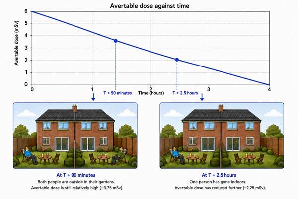
Now imagine two semi-detached houses at a distance downwind that gives an inhalation dose rate of 3.75 mSv an hour for four hours. This translates to half an Emergency Reference Level of dose each hour. (The UK Lower ERL for shelter is 3 mSv dose averted which corresponds to 7.5 mSvv in the open).
As the plume arrives at their homes the projected doses to Mr Blue and Mr Green is 15 mSv comfortably above the action level of 7.5 mSv.
You would recommend that they shelter with some urgency. If they shelter from any time before T + 2 hours they would be assumed to avert more than 3 mSv. The sooner they shelter the better. For example, if Mr Green shelters from T + 1.5 hrs he would avert 3.75 mSv whereas if he sheltered immediately he would avert 6 mSv.
Now consider the situation at T + 2.5 hrs. You become aware that Mr Blue remains in his garden. The avertable dose is now 2.25 mSv. The system would not recommend him to shelter.
But the same system would not recommend that Mr Green break shelter – he is on to avert 3.75 mSv (above the ERL) if he remains in shelter but so far has only averted 1.5 mSv.
We recommend Mr Green stay in shelter but don’t recommend Mr Blue to shelter. Is that the right answer?
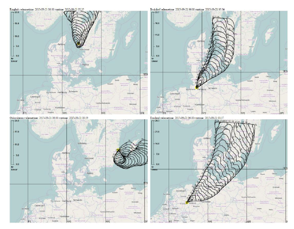
It is common to assess the potential impact of a particular incident at a nuclear power station by estimating a source term for the event and then repeatedly running the source term through an atmospheric dispersion code with different weather conditions to provide a statistical distribution of off-site doses or other impacts.
Met data can be obtained from a variety of sources. These include local observations, nearby (or not so nearby) observations, or synthetic data obtained from the massive weather forecasting and recording models and databases. With improvements in the recording of weather data, synthetic data is increasingly seen as the better option.
Methodologies might run the dispersion code for each line of met data available or may sample the data to reduce computing costs/times but in the hope of the results remaining representative.
What this presentation fails to show is the outlying sequences, met sequences that might be expected to cause high doses further downwind than usual. These include sequences with very low mixing layers and sequences with very low wind speed (see table)
Sequence
Mix Layer/ m
Cat
Wind speed/ m/s
Rainfall
1802
16
F
0.41
0
1803
14
E
0.19
0
1804
17
E
0.49
0
2608
85
B
0.11
0
2698
457
B
0.45
0
2699
268
B
0.5
0
2700
312
B
0.17
0
3921
42
B
0.4
0.317
3951
129
B
0.35
0.05
4090
221
B
0.03
0
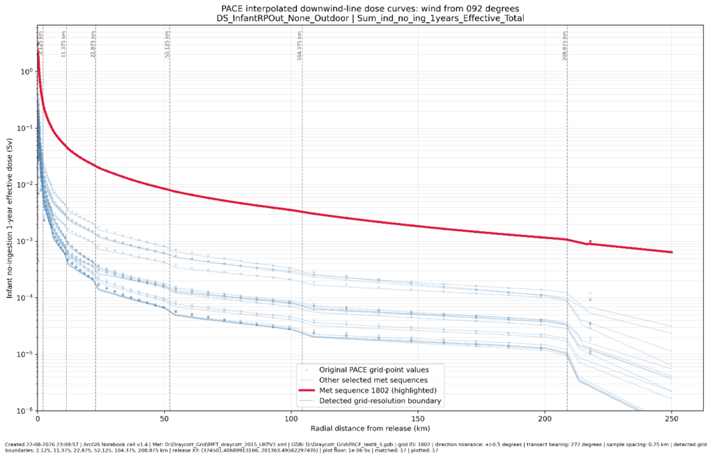
One of these (1802) is for a wind direction of 92 degrees. The figure below shows the dose as a function of downwind distance estimated using the ADEPT R-91 type dispersion code in the PACE model (https://www.ukhsa-protectionservices.org.uk/pace) calculated for all angle with a 92-degree wind direction with sequence 1802 highlighted.
This plot highlights a minor issue with the impact of a change in grid sizes and an issue with the linear interpolation I used to determine the dose at the downwind point of interest (PACE works on a grid rather than your chosen array of points). But it makes the point; there are weather conditions that may produce very different dispersion patterns.
This poses the question “should our emergency planning zones (assuming the source term is accepted as appropriate) be based on the average downwind distance for an exceedance, a high percentile (P95, P98, P100) of the downwind exceedance, or an exceedance by the average dose or a percentile dose at a particular distance”?
UK guidance is to use P95 which should eliminate these outliers (unless your random sample picks up too many of them).
Emergency planners should be aware that an accident could happen on a particularly cold night with very low wind speeds and, if it does, actionable radiation doses might extend much further than expected.
Of course, they might not. With these low wind speeds the penetration of the plume will be very sensitive to deposition (the assumption above is vg=1E-3 m/s) and to changes in the wind speed and direction. Not a good night to depend on your default arrangements or your dispersion code.
I listened to a presentation on the ARGOS (Accident Reporting Guidance and Operational Support – https://pdc-argos.com/index.html) decision support system today (25/08/26).
Their website tells us that ARGOS is useful throughout the entire disaster life cycle:
During the Preparedness phase for planning, dimensioning and training – including evaluation of various ‘What-if’ scenarios
During the Response phase by calculating prognoses about how the situation will evolve; what can be the consequences of the dispersion; what the proper emergency or evacuation zones are; etc.
During the Recovery phase; what will be the effect of applying possible countermeasures; etc.
In the Evaluation phase to study what could have been done better and how could the situation have evolved?
The code is based on the RIMPUFF atmospheric dispersion modelling code (https://inis.iaea.org/records/2mgb1-mfy59) but also has a model optimised for short urban distances (URD – useable for on-site doses, urban dirty bombs and chemical releases).
The code is available from PDC-Argos in Denmark.
Tracing back to 1986 (following Chornobyl) the code has been constantly maintained and updated, new features have been added.
It has customers through out the world.
Its role as a decision support system is to predict where a radioactive plume will go and estimate the projected doses and avertable doses given a possible suite of protective actions.
On the simple interface you pick a location, a source term and a start time from pull down menus (you can add your own site locations and source terms).
You can have up to 1000 release points all with their own source term and time structure.
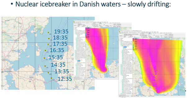
You can model moving sources (see below) which is novel but, with the trend to build floating SMRs and nuclear powered shipping, potentially useful.
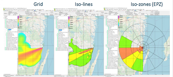
There are various output formats:
You can input data from permanent monitoring stations (including EurDep) , or manual measurements. It is not clear it me how these relate to the dispersion modelling but nonetheless it can be valuable to have measured data and predicted results in the same place.
It does food chain modelling, but to set up for a new region would be a significant amount of work. This allows you to predict where crops may exceed thresholds and for how long that situation would pertain.
You can investigate food countermeasures and land remediation.
You can investigate other dose pathways and how they might vary with time.
You can also now set it up to undertake continuous calculations – automatically work through a whole library of weather data and export to spreadsheet for a statistical analysis of the dose end points.
Automatic running also allows you to have periodic (daily or hourly maybe) predictions of plume arrival times for different source locations.
This seems like a good code to have available in national response centres linked to the national meteorological centre and the national fixed monitor grid, preloaded with NPP locations and a library of sources terms from the safety cases of each. You would then need a skilled operator or two to update the data being fed into the model and interpreting the results and decision makers familiar with the output and the radiological implications of an airborne plume.
The initial role would be radionuclide plume footprint and arrival times (where to apply protective actions), followed by avertable dose as a function of time – checking protective action advice to confirm that it is of sufficient initial extent and is withdrawn in a timely manner.
If you use the code in the planning stage to determine how big the emergency planning zones should be under different circumstances you would gain valuable experience in setting up the code and running it.
It can also be used in exercises, generating off-site radiological conditions for the umpire’s side and modelling the release footprint, arrival time and dose implications for the players.
A useful code for a national response body and a nuclear utility to consider.
This article has been largely written by AI during a conversation lasting about an hour. It seems to me to make sense and the conclusions appear sound. But it for you, the reader, to judge.
1 Purpose
This article describes the basis for the estimates used for the proportion of four population groups — baby/pre-school child, school-age child, adult and elderly person — who would, at different times of day, either already be within a building or be able to reach a substantial building within a specified period.
The estimates were developed for emergency-planning purposes, particularly circumstances in which rapid sheltering may be advised following an atmospheric release. They are derived planning estimates rather than directly observed population statistics. No UK dataset has been identified that directly records the proportion of the population that is, at a particular time, within 5 or 15 minutes of a suitable building.
The estimates therefore combine evidence on:
time spent at home and undertaking different activities;
travel and walking;
age-dependent travel behaviour;
children’s outdoor activity;
outdoor occupations; and
the accessibility of open and green spaces.
The resulting estimates are reproduced in Table 1.
Table 1. Estimated population location relative to accessible substantial buildings
Age group
Period
Already inside
Outside but shelter ≤5 min
Shelter 5–15 min
>15 min from shelter
Shelter ≤15 min
Baby/pre-school
Night
99%
0.5%
0.3%
0.2%
99.8%
Working day
94%
4%
1.5%
0.5%
99.5%
Evening
96%
2.5%
1.0%
0.5%
99.5%
Weekend day
92%
5%
2%
1%
99%
Child
Night
99%
0.5%
0.3%
0.2%
99.8%
School day
94%
4%
1.5%
0.5%
99.5%
Evening
91%
5%
2.5%
1.5%
98.5%
Weekend day
85%
8%
4%
3%
97%
Adult
Night
98%
1%
0.5%
0.5%
99.5%
Working day
86%
7%
4%
3%
97%
Evening
90%
5%
3%
2%
98%
Weekend day
84%
8%
5%
3%
97%
Elderly (65+)
Night
99%
0.5%
0.3%
0.2%
99.8%
Weekday day
93%
4%
2%
1%
99%
Evening
96%
2%
1.5%
0.5%
99.5%
Weekend day
91%
5%
2.5%
1.5%
98.5%
Percentages have been rounded and should not be interpreted as having the statistical precision implied by the individual values.
2 Definition of the location categories
For this assessment a substantial building means a normally occupied or occupiable enclosed building that could provide materially greater protection from an airborne release than remaining outdoors. Houses, schools, offices, shops, public buildings and substantial industrial or commercial premises would normally qualify. Open shelters, lightweight open-sided structures and vehicles have not been assumed to be equivalent to substantial buildings.
Four states were considered:
Already inside: the person is already within a substantial building.
Shelter within 5 minutes: the person is outside but is in a location from which a substantial building could reasonably be entered within approximately five minutes.
Shelter within 5–15 minutes: access is possible but is not immediate.
More than 15 minutes from shelter: the person is in a location or undertaking an activity for which access to a substantial building within approximately 15 minutes cannot reasonably be assumed.
The assessment is consequently not an estimate simply of the fraction of people who are outdoors. This distinction is important. A person walking along an urban street, standing in a school playground or working outside a commercial building is outdoors but may be only seconds or minutes from a substantial building. Such a person is materially different, for emergency-planning purposes, from a hill walker, agricultural worker in a remote field or person on an isolated beach.
3 Adult time-use evidence
The principal evidence concerning the distribution of adult activity through the day was the ONS Time use in the UK: 23 September to 1 October 2023 survey. Participants recorded their activities over complete 24-hour periods. Each participant was allocated one weekday and one weekend diary day. Main activities were recorded in 10-minute periods. The survey therefore provides a useful empirical basis for distinguishing weekday and weekend behaviour and the major components of the day, including sleep/rest, work, household activity, leisure and travel.
The survey does not, however, provide a direct measure of distance or travel time to a suitable building. Time-use evidence was therefore used primarily to constrain the fraction likely to be at home, at work or undertaking other activities, rather than to determine the 5- and 15-minute categories directly.
The very high night-time indoor fractions in Table X.1 follow principally from the dominance of sleep/rest and residential activity during the night. A small residual outdoor fraction was retained to represent night workers, travellers, social/leisure activity and other exceptional circumstances.
Adults were assigned the lowest daytime indoor fraction because this group contains most commuters, outdoor workers and people undertaking travel, shopping, recreation and other activities away from home.
4 Travel
Travel represents one of the principal reasons why a person may not be inside a building at a randomly selected time. The Department for Transport National Travel Survey 2024 (NTS) was therefore used as a second principal evidence source.
The NTS shows substantial travel activity across the population and permits differentiation by age, journey purpose and mode. It was used to constrain the amount of time that could plausibly be assigned to the outdoor and travelling categories.
Travel was not treated as synonymous with inability to shelter. This is an important methodological assumption.
Much travel takes place within built-up areas or between buildings. Similarly, a walking trip does not imply that the pedestrian is remote from shelter. A person walking through a town centre may be outside for an appreciable period while remaining continuously within a minute or two of shops, offices and other buildings.
Consequently, only a fraction of travel activity was allocated to the 5–15-minute category and a still smaller fraction to the >15-minute category. This is a judgement-based allocation rather than an NTS statistic.
5 Children
The principal additional source used for children was the ONS analysis Children’s engagement with the outdoors and sports activities, UK: 2014 to 2015, derived from UK time-use data.
Children aged 8–15 spent an average of 16 minutes per day in parks, countryside, seaside, beach or coastal locations. The corresponding daily participation rate was 12.2%. ONS also found higher average time in these locations at weekends than during weekdays, although the reported difference was not statistically significant.
This evidence was particularly useful because it prevents all children’s leisure or sporting activity from being classified as genuinely remote outdoor activity. Sports and active leisure include activities undertaken indoors and activities undertaken immediately adjacent to buildings.
The child estimates were therefore constructed on the following basis:
night-time occupancy was assumed to be overwhelmingly residential;
school-day occupancy was assumed to be dominated by home and school, both providing immediate building access;
the outdoor fraction was increased during evenings; and
the largest outdoor and remote fraction was assigned to weekend daytime, reflecting greater opportunity for outdoor recreation, sport and countryside activity.
This produced an estimated 3% >15 minutes from a substantial building during weekend daytime, compared with approximately 0.5% during the school day.
The distinction is deliberately conservative because even participation in a park, countryside or coastal activity does not demonstrate that the participant is more than 15 minutes from a building.
6 Babies and pre-school children
There is less direct activity-location evidence for babies and very young children. Their estimates therefore have greater inferential content.
The principal assumption was that babies and pre-school children spend a greater proportion of their time either at home or in childcare, nursery, retail, hospitality or other locations containing buildings. They are also normally accompanied when travelling or undertaking outdoor activity.
A smaller genuinely remote fraction than for school-age children was consequently assigned.
Weekend daytime was again assigned the largest outdoor component, giving an estimated 1% >15 minutes from a building. The estimate is intended to encompass family countryside recreation, beaches, parks and other activities away from buildings.
No claim is made that the 1% value has been directly measured.
7 Elderly population
Older people were assigned high building-accessibility fractions because employment and commuting become progressively less important with age and a greater proportion of activity is residential.
The NTS age breakdown was used qualitatively in making this judgement because it demonstrates substantial changes in journey purpose and mode with age. It also prevents the erroneous assumption that elderly people are almost continuously at home: shopping, personal business, social activity and recreational walking remain important activities amongst older groups.
Accordingly, the estimates allow an appreciable daytime outdoor/travelling fraction while retaining a comparatively small >15-minute fraction. The estimated latter fraction ranges from approximately 0.2% at night to 1–1.5% during daytime/weekend periods.
8 Outdoor occupations
Outdoor employment was specifically considered because it could otherwise result in an underestimate of the adult weekday exposed population.
HSE identifies occupations involving significant outdoor exposure including farm workers, construction workers, market gardeners, outdoor-activity workers and some public-service workers.
ONS also provides Annual Population Survey employment estimates at four-digit occupational classification and four-digit industry level, including breakdowns by age and country. This confirms that sufficiently detailed employment data exist to identify occupational groups with a significant outdoor component.
Outdoor employment was nevertheless not equated with remoteness from buildings. Conceptually, the contribution from an occupation was considered as:
occupational prevalence × fraction of working time outdoors × fraction of outdoor working time remote from a suitable building.
For example, agricultural and forestry work can place workers appreciable distances from buildings and was therefore regarded as contributing disproportionately to the >15-minute category.
Construction workers may also spend a substantial fraction of their working day outdoors, but construction sites frequently contain completed or partly completed buildings, site offices, welfare accommodation and adjacent development. Their probability of being outdoors is therefore substantially greater than their probability of being more than 15 minutes from any usable building.
This distinction was one reason why a relatively large outdoor component could coexist with the comparatively small 3% adult weekday >15-minute estimate.
9 Open-space accessibility
A further plausibility check was provided by Defra’s 2026 Access to green and blue space in England statistics.
Defra defines its “15-minute commitment” in terms of access by walking route to specified green/blue spaces. It reports that 80% of households in England have access to at least one qualifying green or blue space within a 15-minute walk, increasing to 91% for rural households and decreasing to 78% for urban households.
These statistics cannot simply be inverted to calculate distance from a building. They nevertheless provide a useful spatial plausibility check.
In particular, they demonstrate that a large amount of access to parks, paths and other outdoor space occurs directly from the built environment. Consequently, categorising everyone engaged in outdoor recreation as being remote from buildings would substantially overstate the population unable to shelter rapidly.
The Defra evidence was therefore used qualitatively to constrain, rather than directly calculate, the >15-minute fractions.
10 Construction of the estimates
The entries in Table 1 were produced sequentially.
First, a central estimate was made of the fraction already within buildings, using the time-of-day activity pattern appropriate to each age group.
Second, the residual outdoor/travelling population was divided between locations expected to have immediate building accessibility and locations involving progressively greater separation from buildings.
Third, NTS travel evidence was used to check that the outdoor/travelling fraction was compatible with observed levels of travel.
Fourth, the child estimates were checked against the ONS outdoor-activity evidence.
Fifth, the adult weekday estimate was increased relative to the other groups to accommodate outdoor occupations and work-related travel.
Sixth, the weekend child and adult fractions were increased to represent outdoor recreation.
Finally, the estimates were checked against the Defra spatial-access evidence to ensure that outdoor recreation had not implicitly been treated as synonymous with remoteness from buildings.
The method is therefore best described as a constrained expert-judgement model rather than a statistical derivation.
11 Uncertainty and conservatism
There are two different types of uncertainty in Table 1.
The first concerns the fraction already inside a building. This is reasonably well constrained by time-use, employment and travel evidence, although there remains uncertainty concerning the precise definition of indoor activity.
The second, and substantially larger, uncertainty concerns the division of the outdoor population between the ≤5-minute, 5–15-minute and >15-minute categories. No identified national survey measures these quantities directly.
Consequently, values such as:
Adult, working day: 86% inside, 7% within 5 minutes, 4% within 5–15 minutes and 3% beyond 15 minutes
should not be interpreted as measurements with percentage-point precision. A more appropriate interpretation is that the evidence indicates an indoor fraction of approximately 85–90%, while expert judgement suggests that most of the residual population remains close to buildings and only a few percent is likely to be genuinely remote.
For this reason, where the purpose is emergency-planning modelling rather than demographic analysis, a simpler assumption is preferable.
The detailed analysis indicates central estimates of approximately 97–99+% of the population able to obtain access to a substantial building within 15 minutes, depending upon age and time of day.
A generic assumption of:
95% able to obtain substantial shelter within 15 minutes
was therefore proposed as a deliberately conservative planning value.
This 95% value is not an ONS, DfT, HSE or Defra statistic. It is a modelling assumption derived from the evidence described above and incorporates an allowance for uncertainty.
12 Limitations
The estimates are intended to characterise a generic UK population. They should not automatically be applied to a particular site without considering local circumstances.
The proportion unable to reach shelter rapidly could be higher around locations characterised by extensive:
agricultural land;
moorland or mountains;
beaches and coastline;
large parks or recreational areas;
forestry;
reservoirs and other water-based recreation;
outdoor industrial activity; or
transport infrastructure remote from occupied buildings.
Conversely, the generic estimates are likely to be conservative in densely developed urban areas where people outdoors are generally close to multiple buildings.
The analysis also considers physical access to a building, rather than whether the building is open to the public, whether access would be permitted during an emergency, or the degree of radiological protection actually afforded by the building. These issues would require separate consideration.
13 References
Office for National Statistics (2023).Time use in the UK: 23 September to 1 October 2023. Experimental statistics. The survey used full 24-hour diaries, with participants allocated one weekday and one weekend diary day. ONS — Time use in the UK
Office for National Statistics.Children’s engagement with the outdoors and sports activities, UK: 2014 to 2015. Includes time and participation rates for children aged 8–15 in parks, countryside and coastal locations. ONS — Children’s engagement with the outdoors and sports activities
Department for Transport (2025).National Travel Survey 2024. Used for travel frequency, duration, purpose, mode and age-dependent travel behaviour.
Health and Safety Executive.Outdoor workers and sun exposure. Identifies occupational groups for whom work involves extended periods outdoors, including agricultural and construction workers. HSE — Outdoor workers and sun exposure
Office for National Statistics (2026).Employment by detailed occupation and industry, by sex, age group and country, 2024 and 2025. Annual Population Survey estimates at four-digit occupational and industry classification. ONS — Employment by detailed occupation and industry
Department for Environment, Food & Rural Affairs (2026).Access to green and blue space in England. Official statistics in development; provides walking-route-based measures of access to qualifying open spaces, including the 15-minute commitment. Defra — Access to green and blue space in England
Overall evidential status
The source evidence supports the proposition that most people are either indoors or undertaking activities in locations from which buildings are readily accessible. It does not directly measure building accessibility.
Accordingly, Table 1 should be described as derived planning estimates informed by UK time-use, travel, employment and spatial-access statistics, rather than as measured population fractions. The greatest uncertainty attaches to the allocation of people who are outdoors between the ≤5-minute, 5–15-minute and >15-minute categories.